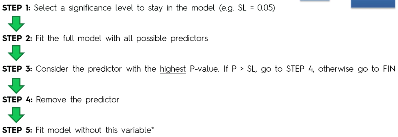
Part 5 Machine Learning Backward Elimination

In the previous post, we learnt about multiple linear regression. The problem with the last approach was that we used all the features without considering that some of the features may not be impacting or playing any role in the outcome. we also talked about 5 ways of reducing the noisy feature. Backward elimination is one of them.

How to get the dataset?

What is `Backward Elimination`?

Backward elimination is a process to remove features that have little effect on the dependent variable.

What could possibly be wrong with leaving the features if they are not impacting or have little impact?

New England Patriots won the Superbowl on Feb 3, 2019. The team won because it had a better team, better skills and a good coach. If I say, the team also won because Patriots fans are great at cheering and that when Patriots play fans supporting the opposition is more tamed, then I would be wrong. If I say that all players in the team wore a white jersey and they won. They also won because they played it on Sunday and T. Brady thinks that it’s his luckiest day. You would call Baloney to all the facts that I just mentioned. It may have helped - may be slightly but too insignificant to make a real difference. The features in a data set are exactly that - Baloney. They only add noise in the actual model and many small non-significant data may actually provide us a model which is way off the margin. The simpler the model, the better the result.

How do we implement `Backward elimination`?

In backward elimination, you take all the variables and create the algorithm. Select a significance level, then consider the predictor with Highest P-value and if P-Value > Significance level then eliminate the variable from the equation, else keep it.
bkwd-elim

How do we implement it in python?

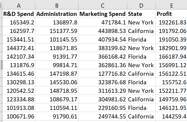
In the previous post, we were trying to figure out if a company is profitable or not by looking at 4 independent variables - R&D Spent, Administration cost, Market spending & State. We created a model with all the features. So let’s pick up from where we left off. Here’s how our dataset looks like
dataset

 1
 2
 3
 4
 5
 6
 7
 8
 9
10
11
12
13
14
15
16
17
18
19
20
21
22
23
24
25
26
27
28
29
30
31
32
33
34
35
36
37
38
39
40
41
42
43
44
45
46
47
48
49


import numpy as np
import matplotlib.pyplot as plt
import pandas as pd

#Read the dataset
dataset = pd.read_csv("50_Startups.csv")

#Divide the dataset in dependent and Independent variables
X= dataset.iloc[:, :-1].values
y = dataset.iloc[:, -1].values



#Taking care of Categorical values.
from sklearn.preprocessing import OneHotEncoder, LabelEncoder
label_encoder = LabelEncoder();
X[:,3]=label_encoder.fit_transform(X[:, 3])
oneHotEncoder = OneHotEncoder(categorical_features=[3])
X= oneHotEncoder.fit_transform(X).toarray()

#getting out of dummy variable trap
X = X[:,1:] # Select all the rows and all the columns starting fom index 1 onwards.
#Create training and test set
from  sklearn.model_selection import train_test_split

X_train, X_test, y_train, y_test = train_test_split(X, y,
                                                    test_size = 0.20,
                                                    train_size=0.80,
                                                    random_state=0)


#Check for missing data
null_columns=dataset.columns[dataset.isnull().any()]
t = dataset[null_columns].isnull().sum()

#Training the model
from sklearn.linear_model import LinearRegression
regressor = LinearRegression()
regressor.fit(X_train, y_train)

# Predicting the results of the training set
y_pred = regressor.predict(X_test)  


print(regressor.coef_)
print(regressor.intercept_)

print('Train Score: ', regressor.score(X_train, y_train))
print('Test Score: ', regressor.score(X_test, y_test))

[-9.59284160e+02  6.99369053e+02  7.73467193e-01  3.28845975e-02
  3.66100259e-02]
42554.16761772438
Train Score:  0.9501847627493607
Test Score:  0.9347068473282446

Take note of Train Score and Test Score

Train Score: 0.9501847627493607

Test Score: 0.9347068473282446

The difference between them is 0.01547791542 or 1.548%

So far we used all the features. Now to use backward elimination we will use an entirely new package and class. However, before we begin, we need to decide on a significance level. In this case, let’s chose a level equal o 0.05.

1
2
3
4


import  statsmodels.formula.api as smf

#Appending ones for constants
X = np.append(arr=np.ones((50,1)).astype(int), values=X, axis=1)

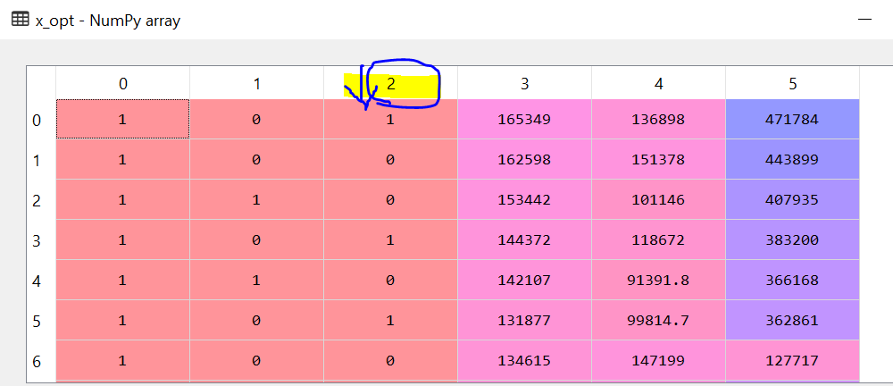
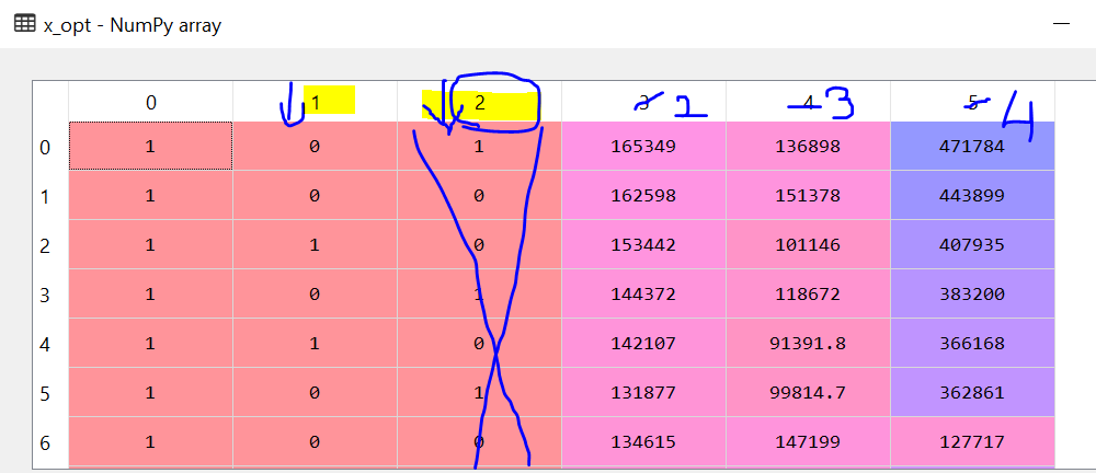
Why did we append 1’s in the existing dataset?

Y = b0X0 + b1X1+ b2X2 + b3X3 + b4X4 + b5X5 + C

In the above equation, if you notice that every X_n has a multiplier b_n but not the constant C. Actually if you have a X₆ and set it to 1 that solves the problem. The question is why do we need a 1 multiplier for the constant. The answer lies in the library and the class that we use. The package statsmodel only considers a multiplier if it has a feature value. If there is no feature value then it would not get picked up while creating the model. So the C would be dropped. Hence we need to create a feature with value = 1.

1
2
3
4


##Creating a model with all varibales
x_opt = X[:,[0,1,2,3,4,5]]
regressor_OLS = smf.OLS(endog=y, exog=x_opt).fit()
print(regressor_OLS.summary())

                            OLS Regression Results                            
==============================================================================
Dep. Variable:                      y   R-squared:                       0.951
Model:                            OLS   Adj. R-squared:                  0.945
Method:                 Least Squares   F-statistic:                     169.9
Date:                Sun, 10 Feb 2019   Prob (F-statistic):           1.34e-27
Time:                        22:42:26   Log-Likelihood:                -525.38
No. Observations:                  50   AIC:                             1063.
Df Residuals:                      44   BIC:                             1074.
Df Model:                           5                                         
Covariance Type:            nonrobust                                         
==============================================================================
                 coef    std err          t      P>|t|      [0.025      0.975]
------------------------------------------------------------------------------
const       5.013e+04   6884.820      7.281      0.000    3.62e+04     6.4e+04
x1           198.7888   3371.007      0.059      0.953   -6595.030    6992.607
x2           -41.8870   3256.039     -0.013      0.990   -6604.003    6520.229
x3             0.8060      0.046     17.369      0.000       0.712       0.900
x4            -0.0270      0.052     -0.517      0.608      -0.132       0.078
x5             0.0270      0.017      1.574      0.123      -0.008       0.062
==============================================================================
Omnibus:                       14.782   Durbin-Watson:                   1.283
Prob(Omnibus):                  0.001   Jarque-Bera (JB):               21.266
Skew:                          -0.948   Prob(JB):                     2.41e-05
Kurtosis:                       5.572   Cond. No.                     1.45e+06
==============================================================================

Based on the process, we now have to find the feature with the highest P-value and if it greater than ould SL then we will drop it. In this case

x2 has the highest P-value = 0.990 > 0.05.

So will drop the feature x2 which corresponds to the State dummy variable
allfeature

We will continue and re-run the model with just 5 feature

1
2
3
4


## Removing index 2 as P>0.05 and is the highest P
x_opt = X[:,[0,1,3,4,5]]
regressor_OLS = smf.OLS(endog=y, exog=x_opt).fit()
print(regressor_OLS.summary())

                            OLS Regression Results                            
==============================================================================
Dep. Variable:                      y   R-squared:                       0.951
Model:                            OLS   Adj. R-squared:                  0.946
Method:                 Least Squares   F-statistic:                     217.2
Date:                Sun, 10 Feb 2019   Prob (F-statistic):           8.49e-29
Time:                        22:52:32   Log-Likelihood:                -525.38
No. Observations:                  50   AIC:                             1061.
Df Residuals:                      45   BIC:                             1070.
Df Model:                           4                                         
Covariance Type:            nonrobust                                         
==============================================================================
                 coef    std err          t      P>|t|      [0.025      0.975]
------------------------------------------------------------------------------
const       5.011e+04   6647.870      7.537      0.000    3.67e+04    6.35e+04
x1           220.1585   2900.536      0.076      0.940   -5621.821    6062.138
x2             0.8060      0.046     17.606      0.000       0.714       0.898
x3            -0.0270      0.052     -0.523      0.604      -0.131       0.077
x4             0.0270      0.017      1.592      0.118      -0.007       0.061
==============================================================================
Omnibus:                       14.758   Durbin-Watson:                   1.282
Prob(Omnibus):                  0.001   Jarque-Bera (JB):               21.172
Skew:                          -0.948   Prob(JB):                     2.53e-05
Kurtosis:                       5.563   Cond. No.                     1.40e+06
==============================================================================

Once again in the above output

x1 has the highest P-value = 0.940 > 0.05

So we will drop X1, which in this case represents the second dummy variable for the State.
allfeature

So we will continue until we don’t have variable that is greater than our significance level

1
2
3
4


## Removing index 1 as P>0.05 and is the highest P
x_opt = X[:,[0,3,4,5]]
regressor_OLS = smf.OLS(endog=y, exog=x_opt).fit()
print(regressor_OLS.summary())

                            OLS Regression Results                            
==============================================================================
Dep. Variable:                      y   R-squared:                       0.951
Model:                            OLS   Adj. R-squared:                  0.948
Method:                 Least Squares   F-statistic:                     296.0
Date:                Sun, 10 Feb 2019   Prob (F-statistic):           4.53e-30
Time:                        22:59:29   Log-Likelihood:                -525.39
No. Observations:                  50   AIC:                             1059.
Df Residuals:                      46   BIC:                             1066.
Df Model:                           3                                         
Covariance Type:            nonrobust                                         
==============================================================================
                 coef    std err          t      P>|t|      [0.025      0.975]
------------------------------------------------------------------------------
const       5.012e+04   6572.353      7.626      0.000    3.69e+04    6.34e+04
x1             0.8057      0.045     17.846      0.000       0.715       0.897
x2            -0.0268      0.051     -0.526      0.602      -0.130       0.076
x3             0.0272      0.016      1.655      0.105      -0.006       0.060
==============================================================================
Omnibus:                       14.838   Durbin-Watson:                   1.282
Prob(Omnibus):                  0.001   Jarque-Bera (JB):               21.442
Skew:                          -0.949   Prob(JB):                     2.21e-05
Kurtosis:                       5.586   Cond. No.                     1.40e+06
==============================================================================

1
2
3
4


## Removing index 1 as P>0.05 and is the highest P
x_opt = X[:,[0,3,5]]
regressor_OLS = smf.OLS(endog=y, exog=x_opt).fit()
print(regressor_OLS.summary())

                            OLS Regression Results                            
==============================================================================
Dep. Variable:                      y   R-squared:                       0.950
Model:                            OLS   Adj. R-squared:                  0.948
Method:                 Least Squares   F-statistic:                     450.8
Date:                Sun, 10 Feb 2019   Prob (F-statistic):           2.16e-31
Time:                        22:59:39   Log-Likelihood:                -525.54
No. Observations:                  50   AIC:                             1057.
Df Residuals:                      47   BIC:                             1063.
Df Model:                           2                                         
Covariance Type:            nonrobust                                         
==============================================================================
                 coef    std err          t      P>|t|      [0.025      0.975]
------------------------------------------------------------------------------
const       4.698e+04   2689.933     17.464      0.000    4.16e+04    5.24e+04
x1             0.7966      0.041     19.266      0.000       0.713       0.880
x2             0.0299      0.016      1.927      0.060      -0.001       0.061
==============================================================================
Omnibus:                       14.677   Durbin-Watson:                   1.257
Prob(Omnibus):                  0.001   Jarque-Bera (JB):               21.161
Skew:                          -0.939   Prob(JB):                     2.54e-05
Kurtosis:                       5.575   Cond. No.                     5.32e+05
==============================================================================

1
2
3
4


## Removing index 1 as P>0.05 and is the highest P
x_opt = X[:,[0,3]]
regressor_OLS = smf.OLS(endog=y, exog=x_opt).fit()
print(regressor_OLS.summary())

                            OLS Regression Results                            
==============================================================================
Dep. Variable:                      y   R-squared:                       0.947
Model:                            OLS   Adj. R-squared:                  0.945
Method:                 Least Squares   F-statistic:                     849.8
Date:                Sun, 10 Feb 2019   Prob (F-statistic):           3.50e-32
Time:                        22:59:43   Log-Likelihood:                -527.44
No. Observations:                  50   AIC:                             1059.
Df Residuals:                      48   BIC:                             1063.
Df Model:                           1                                         
Covariance Type:            nonrobust                                         
==============================================================================
                 coef    std err          t      P>|t|      [0.025      0.975]
------------------------------------------------------------------------------
const       4.903e+04   2537.897     19.320      0.000    4.39e+04    5.41e+04
x1             0.8543      0.029     29.151      0.000       0.795       0.913
==============================================================================
Omnibus:                       13.727   Durbin-Watson:                   1.116
Prob(Omnibus):                  0.001   Jarque-Bera (JB):               18.536
Skew:                          -0.911   Prob(JB):                     9.44e-05
Kurtosis:                       5.361   Cond. No.                     1.65e+05
==============================================================================

So in the end, we find that only the C constant and the R&D Spending are really the important or most significant feature to find out if we should invest in the new business venture.

How do I believe you that by just keeping R&D feature, will improve our model accuracy?

Let’s recalculate our model using the Linear Regression library and find the difference between accuracy score

 1
 2
 3
 4
 5
 6
 7
 8
 9
10
11



import numpy as np
import matplotlib.pyplot as plt
import pandas as pd

#Read the dataset
dataset = pd.read_csv("50_Startups.csv")

#Divide the dataset in dependent and Independent variables
X= dataset.iloc[:, 0].values ##Get the R&D score only
y = dataset.iloc[:, -1].values

1
2
3
4
5
6
7


#Create training and test set
from  sklearn.model_selection import train_test_split

X_train, X_test, y_train, y_test = train_test_split(X, y,
                                                    test_size = 0.20,
                                                    train_size=0.80,
                                                    random_state=0)

 1
 2
 3
 4
 5
 6
 7
 8
 9
10
11
12
13
14


#Training the model
from sklearn.linear_model import LinearRegression
regressor = LinearRegression()
regressor.fit(np.array(X_train).reshape(-1,1), y_train)

# Predicting the results of the training set
y_pred = regressor.predict(np.array(X_test).reshape(-1,1))


print(regressor.coef_)
print(regressor.intercept_)

print('Train Score: ', regressor.score(np.array(X_train).reshape(-1,1), y_train))
print('Test Score: ', regressor.score(np.array(X_test).reshape(-1,1), y_test))

[0.8516228]
48416.297661385026
Train Score:  0.9449589778363044
Test Score:  0.9464587607787219

Let’s look at the Train score and Test Score with all the feature and with just R&D spending.

With all Features
Train Score: 0.9501847627493607 & Test Score: 0.9347068473282446

Difference = 0.01547791542 or 1.548%

With just R&D spending feature
Train Score: 0.9449589778363044 & Test Score: 0.9464587607787219

Difference = 0.0014997829424 or 0.150%

Also the if you see that the test score has improved when from 93.6% to 94.6%.

Hopefully, you enjoyed this series. In the next series, we will look at slightly more interesting topic called SVMs or Support Vector Regression.