Business Goal: As an owner of MuShu Bike Rental CO. in New York. I want to know how many bicycles will be rented on any given day based on daily temperature, humidity and wind speed. Can you help MuShu Bike Rental CO. to predict the number of daily rentals?

How to get the dataset?

• Startup Dataset
• Support vector Regression notebook

Let’s solve this problem using SVR - Support Vector Regression.
Before we begin, let’s see the key terms that will be used.

Key terms

• Kernel

A fancy word for the function used to map a lower dimension data into higher dimension data.

• Hyper Plane

This is a line that helps us predict the target values.

• Boundary Line

There are two boundary lines which separate the classes. The support vectors can be on the boundary line or outside the boundary line.

• Support Vectors

Support vectors are the data points which are closest to the boundary line.

What is a SVR model?

In Simple/multiple regression we try to minimize the errors while in SVR, we try to fit the error within a threshold.

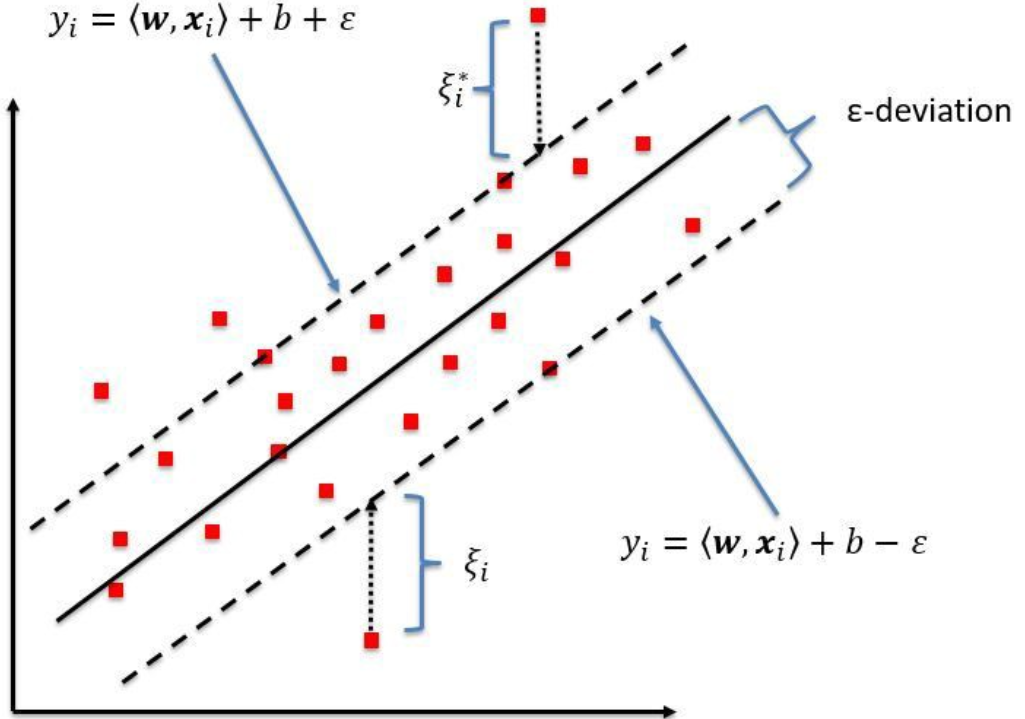
Blue Line: Hyper Plane | Red Line: Boundary lines

Looking at the above figure, our goal is to have the data points inside the boundary lines and hyperplane with the maximum number of data points.

What is “Boundary again?

The red lines that you see in the diagram above are called boundary lines. These lines are at equidistant from a hyper plane (Blue line). So basically, if one boundary line is at distance “e” distance from a hyper plane the other would be at distance of "-e”.
In mathematical equation.
If the hyper plane line is a straight line going through Y-AXIS and represented as

mX + C =0

Then the equation of boundary lines can be represented as

mX + C = e
mx +C = -e

The final equation of SVR can be represented as

e≤ y-mx-c ≤+e

To summarize: The goal so far is to find the distance value e which is equidistant from hyper plane line with the maximum data points OR that they are inside the Boundary line.

Exploring the dataset

1
2
3
4
5
6

import numpy as np
import pandas as pd
import matplotlib.pyplot as plt

##Import the datset
dataset = pd.read_csv('BikeRental/bike_rental_train.csv')

1

dataset.head()

1

dataset.describe().T

1

dataset.columns

Index(['temp', 'humidity', 'windspeed', 'bike_rent_count'], dtype='object')

1

plt.scatter( dataset.temp, dataset.bike_rent_count, c='green');

1

plt.scatter( dataset.humidity,dataset.bike_rent_count);

1

plt.scatter( dataset.windspeed, dataset.bike_rent_count);

Summary
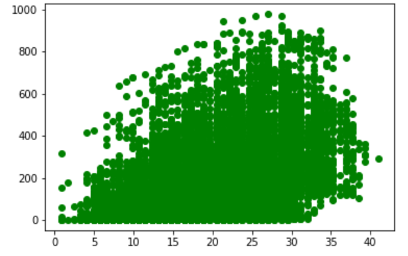
Based on data description and histogram plot.

• Temp Range = 0 to 41
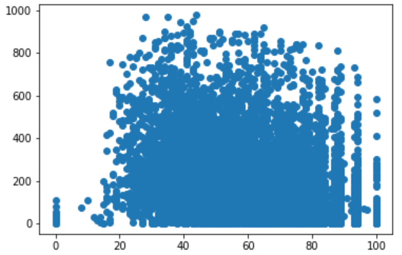
• Humidity Range = 0 to 100
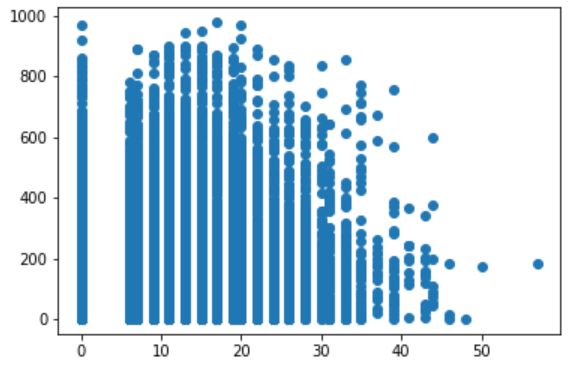
• Windspeed = 0 to 57

1

dataset.corr(method='pearson', min_periods=1)

Summary

• Looking at the correlation matrix, we see that there is a positive relationship between temperature and bike_rent_count
• Humidity has a negative effect on bike_rent_count. Higher the humidity, lower the number of rentals
• Windspeed has little effect on bike_rent_count.
  Looking at the correlation matrix, it confirms the visuals that bike count rental has a weak correlation with all of the 3 variables.

What does a weak correlation mean?
It means that the equation of the model that we are going to plot is probably not going to give very accurate results. However, the goal of this post is to show you how to implement SVR.

So Let’s bring out our template from our first post on data pre-processing.

Step 1: Let’s break the data into Dependent and Independent variable

1
2
3

### Break up in dependent and Independent variables
X = dataset.iloc[:, 0:3].values
y = dataset.iloc[:, 3].values

Step 2 : Break the data into train and test set

1
2
3

# Splitting the dataset into the Training set and Test set
from sklearn.model_selection import train_test_split
X_train, X_test, y_train, y_test = train_test_split(X, y, test_size = 0.2, random_state = 0)

Step 3: Feature scaling. This step is required here beacause SVR library does not do feature scaling.

1
2
3
4
5
6
7

# Feature Scaling
from sklearn.preprocessing import StandardScaler
sc_X = StandardScaler()
X_train = sc_X.fit_transform(X_train)
X_test = sc_X.transform(X_test)
#sc_y = StandardScaler()
#y_train = sc_y.fit_transform(y_train)

Step 4: Create a Regressor and fit the model

1
2
3
4
5
6

# Fitting the SVR Model to the dataset
from sklearn.svm import SVR

# Create your regressor here
regressor = SVR(kernel='linear')
regressor.fit(X_train,y_train)

SVR(C=1.0, cache_size=200, coef0=0.0, degree=3, epsilon=0.1,
  gamma='auto_deprecated', kernel='linear', max_iter=-1, shrinking=True,
  tol=0.001, verbose=False)

In the above code, we are using the SVR class for fitting the model.

SVR(
[“kernel=‘rbf’”, ‘degree=3’, “gamma=‘auto_deprecated’”, ‘coef0=0.0’, ’tol=0.001’, ‘C=1.0’, ’epsilon=0.1’, ‘shrinking=True’, ‘cache_size=200’, ‘verbose=False’, ‘max_iter=-1’],
)

The SVR model that we are using provides 4 types of Kernel - rbf, linear, poly, sigmoid. In our case, we are using linear since data appears to be linear based on visualizations. Another interesting attribute is verbose, which when set to true will show you the default values used of other attributes.

Step 5: Predict the bike count based on test data

1
2

# Predicting a new result
y_pred = regressor.predict(X_test)

Step 6: Check the model effeciency

1
2

print('Train Score: ', regressor.score(X_train, y_train))
print('Test Score: ', regressor.score(X_test, y_test))

Train Score:  0.19926232721567205
Test Score:  0.2082800818663224

As mentioned earlier, since the correlation is weak, we can see that our model is extremely weak. One thing to note here is that I downloaded this random dataset from some website. So when I was working on SVR, I was not sure if the data is true or not.

Let’s try the tweaking SVR model a little to see if we can do better.

 1
 2
 3
 4
 5
 6
 7
 8
 9
10
11
12
13
14
15

# Create your regressor here
regressor = (SVR(kernel='poly',
                 shrinking=True,
                  degree=7,
                gamma='scale',
                 epsilon = 0.01,
                 coef0 =1.60
                ))
regressor.fit(X_train,y_train)

# Predicting a new result
y_pred = regressor.predict(X_test)

print('Train Score: ', regressor.score(X_train, y_train))
print('Test Score: ', regressor.score(X_test, y_test))

Train Score:  0.25167703525198526
Test Score:  0.2484248213345378

So after playing around with different option and values, you will see that if you use poly or polynomial kernel, I was able to push the model prediction to 25.xx%.

So that’s it for this series. Try a different dataset, probably get one from the Multiple Linear regression about 50_Startups and predict using linear kernel.

In the next series, we will learn about our first ever classification model - Decision Trees. Till then happy Happy hyper-planing